11. Event Detection

An event is some phenomena that has a distinct temporal pattern. In the simplest case there is a distinct start of the event (often called an onset), and a distinct end of the event (offset). But sometimes the end (or start) is a gradual or indistinct transition. More rarely, both the start and end are gradual - like the sound of a car passing by.

Often we are interested in detecting the time when the events start and end, counting the number of events, calculating the event durations, and sometimes classifying the type of event. This need for fine-grained information about start/end time and discrete (countable) events, is one of the key elements that separates event detection from standard classification.

Event Detection is usually approached as a supervised learning task, and requires that the dataset has a labeled set of events (with start, end and class).

11.1. Applications

Detecting events using Machine Learning has a wide range of applications, and it is commonly performed on sensor data using embedded systems.

Application examples
Area	Task	Sensor
Ecology	Birdcall detection	Sound
Music	Note onset detection	Sound
Speech	Voice Activity Detection	Sound
Health	Gait tracking during walking	Accelerometer
Health	Heart rate monitoring	Optical reflectometer
Health	Epelepsy seizure	EEG
Health	Sleep apnea event detection	Accelerometer

11.2. Binary or multi-class

Event Detection is often binary (the target event is either present or not), but it may also be multi-class (multiple event types that can each be present or not). In a multi-class setting, all the event classes can be handled by a single multi-class detector, or each event class can be modeled using an independent binary event detector model.

11.3. Sliding time windows

The continuous input time-series data is usually transformed into a series of fixed-length feature vectors. Individual features vector for one time-step is often referred to as a frame. Multiple frames are often combined to form a context window, consisting of N frames. This is often referred to as using sliding windows or moving windows, or using a continious classification approach.

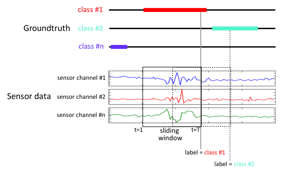
_images/event_detection_labels_windows.png — The training setup for Event Detection as a continious classification problem. The input sensor data is split into fixed-length windows, and the label comes from the event annotations. Image source: “Deep Convolutional and LSTM Recurrent Neural Networks for Multimodal Wearable Activity Recognition” (Roggen et al., 2016)

The distance between windows is known as the hop length. This is normally smaller than the size of the window (window length), so effectively there is a degree of overlap between consecutive windows. The overlap might be as low as 50%, or as high as 99%. This ensures that the model sees the events during training at multiple different positions inside the window. And a high overlap during inference can give multiple predictions per event, which can be merged together to give a better estimate than a single prediction.

The window length is an important hyperparameter for event detection, and is preferably tuned through to the task at hand via experimentation. A good starting point is that windows are large enough to easily cover the transition between event and not (onset/offset).

The hop length decides the time resolution of the output predictions/activations, and must be set based on the precision requirements for the task.

The sliding-window computation is usually done in combination with Feature extraction.

11.4. Classification models for Event Detection

The use of the sliding window approach in combination with feature engineering makes it possible to use any standard machine learning classifier for event detection. For an overview of available classifiers see Classification.

11.5. Training with class imbalance

Event detection problems usually have a considerable class imbalance: Events are usually quite rare versus no-event. This may need to be accounted for during training to get a well performing model.

One approach is to balance the classes. This is done either by oversampling the minority class, undersampling the majority class, or a combination. The imbalanced-learn library provides tools for this.

Some models also support adjusting the optimization objective in ways that can be used to counteract class imbalance problems. This can be in terms of a class weights or sample weights. Examples of models supported by emlearn with these capabilities are RandomForest, and keras.Sequential.

11.6. Trade-off between False Alarms and Missed Detections

Event Detection involves a binary decision problem (is it an event or not), has an inherent trade-off between False Alarms and Missed Detections. Different usecases and applications often have a different preference for the preferred balance between these two.

It is useful to visualize the trade-offs that are possible for a given model/system. There are a number of standard plots used for this purpose, such as:

Detection Error Trade-off (DET) curve
Receiver Operating Characteristic (ROC) curve
Precision-Recall (PR) curve

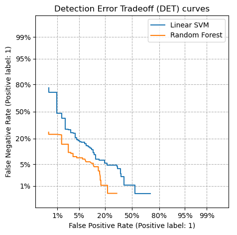
_images/detection_error_tradeoff_curve.png — A Dection Error Curve (DET) is useful to visualize the tradeoff between False Positive and False Negative, as well as compare the performance of multiple models against eachother.

scikit-learn has utilities to produce these, with several examples on Precision-Recall curves and DET and ROC curves.

The operating point along such a curve is set by applying a decision threshold on top of a continuous output. Most classification models in emlearn support such a continuous output with a predict_proba() function.

11.7. Evaluation metrics

There are several evaluation metrics that are commonly used for event detection.

Some compare performance at a particular operating point / threshold:

F-score (F1, F-beta, etc.)
Precision/Recall
False Positive Rate (FPR) / False Negative Rate (FNR)
False Acceptance Rate (FAR) / False Rejection Rate (FRR)

Others compare performance across the operating range:

Area Under Curve Precision-Recall (AUC-PR)
Average Precision (AP)

Metrics may be computed either per frames or analysis window (frame-wise), or event-wise.

11.8. Frame-wise evaluation

Frame-wise evaluation is readily done using the standard metrics, as each frame or window is one instance/sample for the model to predict on, and the prediction is compared with its corresponding label in the same way as standard classification.

However sometimes we do not need each and every frame to be correct. For example we may tolerate a bit of slop in the onset and offset. Especially since the groundtruth labels themselves may have some imprecision. In the case, the results of frame-wise evaluation may underestimate practical performance.

11.9. Event-wise evaluation

Event-wise evaluation is often closer to the practical performance. It allows to specify some tolerance in time, and whether to evaluate only based on onsets, or also offsets/duration. However, event-wise evaluation is not as commonly supported in standard machine learning toolkits. But one can implement it using a module such as sed_eval.