Note
Go to the end to download the full example code.
Optimizing model size for trees
Example of hyperparameter-optimization of a tree-based classifier model.
When optimizing a model that will be ran on an embedded device, we usually want to optimize not just the predictive performance (given by our metric, say accuracy) but also the computational costs of the model (in terms of storage, memory and CPU requirements).
emlearn provides tools for analyzing model costs in the emlearn.evaluate submodule.
This is an example of how to do that, by optimizing hyperparamters using random search, and finding the models that represent good performance/cost trade-offs (Pareto optimimal). The search optimizes the two main things that influence performance and cost: the number of decision nodes in the trees (the depth), and the number of trees in the ensemble (the “breath” of the model).
This method is simple and a good starting point for a broad search of possible models. However if you have a large dataset, consider reducing subsampling the training-set to speed up search.
import os.path

import emlearn
import numpy
import pandas
import seaborn
import matplotlib.pyplot as plt

try:
    # When executed as regular .py script
    here = os.path.dirname(__file__)
except NameError:
    # When executed as Jupyter notebook / Sphinx Gallery
    here = os.getcwd()


from emlearn.examples.datasets.sonar import load_sonar_dataset, tidy_sonar_data
Load dataset
The Sonar dataset is a basic binary-classification dataset, included with scikit-learn Each instance constains the energy across multiple frequency bands (a spectrum).
data = load_sonar_dataset()
tidy = tidy_sonar_data(data)
tidy.head(3)
Visualize data
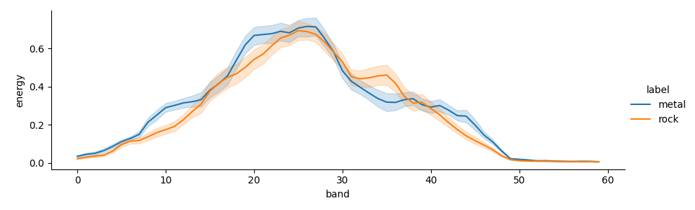
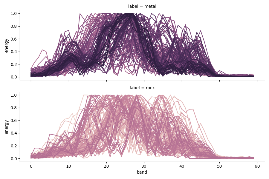
Looking at the overall plot, the data looks easily separable by class. But plotting each sample shows that there is considerable intra-class variability.
seaborn.relplot(data=tidy, kind='line', x='band', y='energy', hue='label',
        height=3, aspect=3)


seaborn.relplot(data=tidy, kind='line', x='band', y='energy', hue='sample',
            row='label', ci=None, aspect=3, height=3, legend=False);
/home/docs/checkouts/readthedocs.org/user_builds/emlearn/envs/stable/lib/python3.12/site-packages/seaborn/axisgrid.py:854: FutureWarning:

The `ci` parameter is deprecated. Use `errorbar=None` for the same effect.

  func(*plot_args, **plot_kwargs)
/home/docs/checkouts/readthedocs.org/user_builds/emlearn/envs/stable/lib/python3.12/site-packages/seaborn/axisgrid.py:854: FutureWarning:

The `ci` parameter is deprecated. Use `errorbar=None` for the same effect.

  func(*plot_args, **plot_kwargs)

<seaborn.axisgrid.FacetGrid object at 0x710ca8a94f80>
Setup model evaluation and optimization
Using RandomizedSearchCV from scikit-learn for random search of hyperparameters. In addition to a standard accuracy metric to estimate the predictive performance of the model, we use two functions from emlearn.evaluate.trees to estimate the storage and compute requirements of the model. The outputs will be used to identify models that offer a good tradeoff between predictive performance and compute costs (Pareto optimal).
from sklearn.ensemble import RandomForestClassifier
from sklearn.model_selection import train_test_split
from sklearn.preprocessing import LabelEncoder
from sklearn.metrics import accuracy_score
import sklearn.model_selection

# custom metrics for model costs
from emlearn.evaluate.trees import model_size_bytes, compute_cost_estimate


def evaluate_classifier(model, data, features=None, cut_top=None):
    spectrum_columns = [c for c in data.columns if c.startswith('b.')]

    if features is None:
        features = spectrum_columns
    if cut_top is not None:
        features = features[:-cut_top]

    # minimally prepare dataset
    X = data[features]
    y = data['label']
    X = X.astype('float32')
    y = LabelEncoder().fit_transform(y.astype('str'))
    # split into train and test sets
    X_train, X_test, y_train, y_test = train_test_split(X, y, test_size=0.33, random_state=1)

    # perform the search
    model.fit(X_train, y_train)
    # summarize
    y_hat = model.predict(X_test)
    acc = accuracy_score(y_test, y_hat)
    print("Accuracy: %.3f" % acc)

def build_hyperparameter_optimizer(hyperparameters={}, cv=10, n_iter=100, n_jobs=-1, verbose=1):

    search = sklearn.model_selection.RandomizedSearchCV(

        RandomForestClassifier(n_jobs=1),

        param_distributions=hyperparameters,
        scoring={
            # our predictive model metric
            'accuracy': sklearn.metrics.make_scorer(sklearn.metrics.accuracy_score),

            # metrics for the model costs
            'size': model_size_bytes,
            'compute': compute_cost_estimate,
        },
        refit='accuracy',
        n_iter=n_iter,
        cv=cv,
        return_train_score=True,
        n_jobs=n_jobs,
        verbose=verbose,
    )

    return search
Build a baseline model
Uses the default hyper-parameters for scikit-learn RandomForestClassifier, not searching any alternatives. This is our un-optimized reference point.
baseline = build_hyperparameter_optimizer(hyperparameters={}, n_iter=1) # default
evaluate_classifier(baseline, data)
baseline_results = pandas.DataFrame(baseline.cv_results_)
baseline_results[['mean_test_accuracy', 'mean_test_size', 'mean_test_compute']]
Fitting 10 folds for each of 1 candidates, totalling 10 fits
Accuracy: 0.783
Optimize hyper-parameters
The number of trees in the decision forest is optimized using the parameter n_estimators. Multiple strategies are shown for limiting the depth of the trees, using either max_depth, min_samples_leaf, min_samples_split or ccp_alpha.
To keep running the example fast, we only do a limited number of different hyper-parameters (controlled by n_iterations). Better results are expected if increasing this by factor 10-100x.
import scipy.stats

def run_experiment(depth_param=None, n_iter=1):
    import time

    start_time = time.time()

    optimize_params = [
        'n_estimators',
        depth_param,
    ]

    print('Running experiment: ', depth_param)

    hyperparams = { k: v for k, v in parameter_distributions.items() if k in optimize_params }

    search = build_hyperparameter_optimizer(hyperparams, n_iter=n_iter, cv=5)
    evaluate_classifier(search, data)
    df = pandas.DataFrame(search.cv_results_)
    df['depth_param_type'] = depth_param
    df['depth_param_value'] = f'param_{depth_param}'

    end_time = time.time()
    duration = end_time - start_time
    print(f'Experiment took {duration:.2f} seconds', )

    df.to_csv(f'sonar-tuning-results-{depth_param}-{n_iter}.csv')

    return df

# Spaces to search for hyperparameters
parameter_distributions = {
    # regulates width of the ensemble
    'n_estimators': scipy.stats.randint(5, 100),

    # different alternatives to regulates depth of the trees
    'max_depth': scipy.stats.randint(1, 10),
    'min_samples_leaf': scipy.stats.loguniform(0.01, 0.33),
    'min_samples_split': scipy.stats.loguniform(0.01, 0.60),
    'ccp_alpha': scipy.stats.uniform(0.01, 0.20),
}

# Experiments to run, using different ways of constraining tree depth
depth_limiting_parameters = [
    'max_depth',
    'min_samples_leaf',
    'min_samples_split',
    'ccp_alpha',
]

# Number of samples to try for different hyper-parameters
n_iterations = int(os.environ.get('EMLEARN_HYPER_ITERATIONS', 1*100))

results = pandas.concat([ run_experiment(p, n_iter=n_iterations) for p in depth_limiting_parameters ])
results.sort_values('mean_test_accuracy', ascending=False).head(10)[['mean_test_accuracy', 'mean_test_size', 'mean_test_compute']]
Running experiment:  max_depth
Fitting 5 folds for each of 100 candidates, totalling 500 fits
Accuracy: 0.768
Experiment took 25.86 seconds
Running experiment:  min_samples_leaf
Fitting 5 folds for each of 100 candidates, totalling 500 fits
Accuracy: 0.841
Experiment took 24.13 seconds
Running experiment:  min_samples_split
Fitting 5 folds for each of 100 candidates, totalling 500 fits
Accuracy: 0.797
Experiment took 26.70 seconds
Running experiment:  ccp_alpha
Fitting 5 folds for each of 100 candidates, totalling 500 fits
Accuracy: 0.783
Experiment took 20.40 seconds
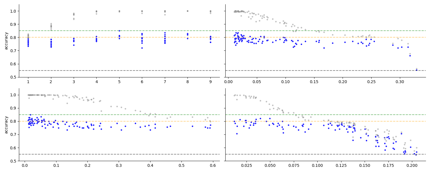
Check effect of depth parameter
The different values of the hyperparamterer affecting tree depth influence the regularization considerably. One can see that for certain values there is overfitting (train accuracy near 100%, far above test), and for other values there is a underfitting (train accuracy near test, and test dropping). This means that our search space is at wide enough to cover the relevant area.
Note that n_estimators is also varied and affects the results, but is not visualized here.
def add_performance_references(ax):
    ax.axhline(0.55, ls='--', alpha=0.5, color='black')
    ax.axhline(0.85, ls='--', alpha=0.5, color='green')
    ax.axhline(0.80, ls='--', alpha=0.5, color='orange')

def plot_scores(data, color=None, metric='accuracy', s=10):
    ax = plt.gca()
    x = 'param_' + data['depth_param_type'].unique()[0]

    seaborn.scatterplot(data=data, x=x, y=f'mean_test_{metric}', alpha=0.9, color='blue', label='test', s=s)
    seaborn.scatterplot(data=data, x=x, y=f'mean_train_{metric}', alpha=0.5, color='grey', label='train', s=s)

    add_performance_references(ax)
    ax.set_ylim(0.5, 1.05)
    ax.set_ylabel('accuracy')
    ax.set_title('')
    ax.set_xlabel('')

g = seaborn.FacetGrid(results, col='depth_param_type', col_wrap=2, height=3, aspect=2.5, sharex=False)
g.map_dataframe(plot_scores, s=15);
<seaborn.axisgrid.FacetGrid object at 0x710ca91fb2c0>
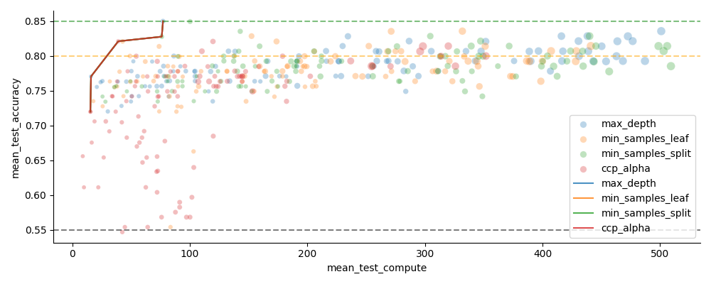
Trade-off between predictive performance and model costs
There will always be a trade-off between how well a model does, and the costs of the model. But it is only worth considering the models that for a given performance level, have better (lower) cost. The models that fulfill this are said to lie on the Pareto front, or that they are Pareto optimal.
In the below plot: The primary model cost axis has been chosen as the (estimated) compute time, shown along the X axis. Model size is considered secondary, and is visualized using the size of the datapoints. The Pareto optimal models, for each depth limiting strategy, is highlighted with lines.
from emlearn.evaluate.pareto import plot_pareto_front, find_pareto_front

def plot_pareto(results, x='mean_test_compute', **kwargs):
    g = plot_pareto_front(results, cost_metric=x, pareto_global=True, pareto_cut=0.7, **kwargs)
    ax = plt.gca()
    add_performance_references(ax)
    ax.legend()

# sphinx_gallery_thumbnail_number = 4
plot_pareto(results, hue='depth_param_type', height=4, aspect=2.5)
Summarize Pareto-optimal models
Compared to the baseline, the optimized models are many times smaller and execute many times faster, while matching or exceeding performance.
pareto = find_pareto_front(results, min_performance=0.7)
ref = baseline_results.iloc[0]
rel = pareto.copy()
rel = pandas.concat([pareto, baseline_results])
# compute performance relativeto baseline
rel['accuracy'] = (rel['mean_test_accuracy'] - ref['mean_test_accuracy']) * 100
rel['compute'] = ref['mean_test_compute'] / rel['mean_test_compute']
rel['size'] = ref['mean_test_size'] / rel['mean_test_size']
rel = rel.sort_values('accuracy', ascending=False).round(2).reset_index()
rel[['accuracy', 'compute', 'size']]
Total running time of the script: (1 minutes 42.662 seconds)